Combined student analysis
Task 7 · 16 students, support and readiness
Everything together: data checks, pooled and stratified rates, weights, a common mix, one histogram and a written conclusion that separates association from causation.
Lab 6 PDF pp. 7–8 · Task 7 (30 minutes)
Your task
Check the 16 rows, compute pooled and within-readiness pass rates, reconstruct them with weights, compare a 50:50 mix, describe your assigned group's distribution, and write a 4–6 sentence conclusion.
Evidence to include
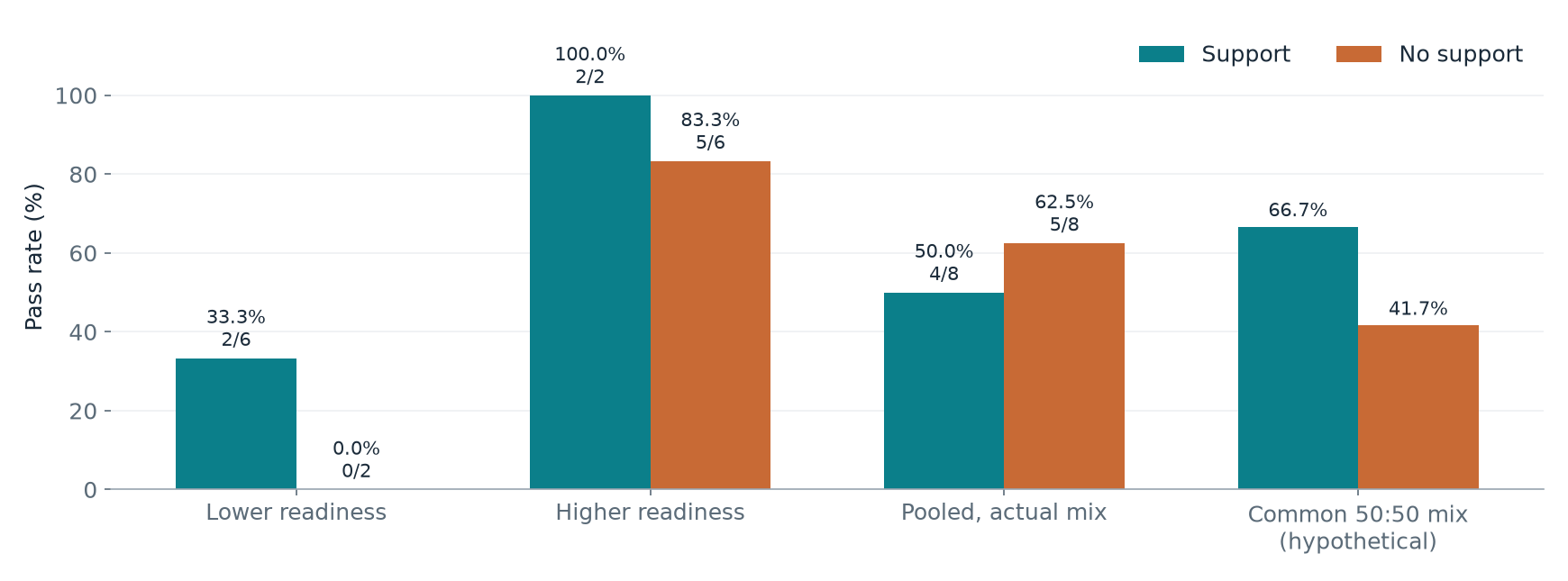
Pooled 4/8 = 50% versus 5/8 = 62.5%; within readiness 2/6 vs 0/2 and 2/2 vs 5/6; weights 0.75/0.25; common-mix 66.7% vs 41.7%; your group's n, mean, median and range.
Worked example and code
Try the task in the PDF first, then compare your working below. Run the code in your own Python notebook.
Open Lab 6 instructions (PDF)Task 7 · L6 pp. 7–8.
1. Enter and check the table
rows = [
    ["S01","Yes","Lower",40], ["S02","Yes","Lower",45],
    ["S03","Yes","Lower",50], ["S04","Yes","Lower",55],
    ["S05","Yes","Lower",35], ["S06","Yes","Lower",48],
    ["S07","Yes","Higher",72], ["S08","Yes","Higher",82],
    ["S09","No", "Lower",30], ["S10","No", "Lower",44],
    ["S11","No", "Higher",49], ["S12","No", "Higher",60],
    ["S13","No", "Higher",65], ["S14","No", "Higher",70],
    ["S15","No", "Higher",80], ["S16","No", "Higher",90]]
df = pd.DataFrame(rows, columns=["id", "support", "readiness", "grade"])
df["passed"] = df["grade"] >= 50
print("Rows:", len(df), "Unique IDs:", df["id"].nunique(),
      "Missing grades:", df["grade"].isna().sum())
print(df["support"].value_counts())
Output: Rows: 16 Unique IDs: 16 Missing grades: 0; Yes 8, No 8. S03's grade of 50 is a pass; S11's 49 is not.
2. Predict by hand
Support = Yes passes: S03, S04, S07, S08 → 4/8. Support = No passes: S12–S16 → 5/8. Prediction: no support leads overall, but within readiness levels support may lead because most supported students are lower-readiness.
3. Pooled and within-readiness rates
overall = df.groupby("support")["passed"].agg(["sum", "count"])
overall["rate_pct"] = 100 * overall["sum"] / overall["count"]
print(overall)
within = df.groupby(["readiness", "support"])["passed"].agg(["sum", "count"])
within["rate_pct"] = 100 * within["sum"] / within["count"]
print(within)
| Readiness | Support: passes/n | No support: passes/n |
|---|---|---|
| Lower | 2/6 = 33.3% | 0/2 = 0.0% |
| Higher | 2/2 = 100.0% | 5/6 = 83.3% |
| Pooled | 4/8 = 50.0% | 5/8 = 62.5% |
Overall gap (support − no support) = 50.0 − 62.5 = −12.5 percentage points. Within lower readiness support leads by +33.3 points; within higher readiness by +16.7 points. The ranking reverses: Simpson's paradox. Six of the eight supported students are lower-readiness, versus two of the eight unsupported students, and lower-readiness students pass far less often.
4. Weights and a common mix
- Support: lower weight 6/8 = 0.75, higher weight 2/8 = 0.25. (6/8)×(2/6) + (2/8)×(2/2) = 0.25 + 0.25 = 0.50.
- No support: lower weight 2/8 = 0.25, higher weight 6/8 = 0.75. (2/8)×(0/2) + (6/8)×(5/6) = 0 + 0.625 = 0.625.
Both reconstructions equal the pooled rates, and each pair of weights sums to 1.
Common 50:50 readiness mix:
- Support: 0.5 × 33.3% + 0.5 × 100% = 66.7%.
- No support: 0.5 × 0% + 0.5 × 83.3% = 41.7%.
The observed pooled rate describes the groups as they actually are, with different readiness mixes. The common-mix rate answers a hypothetical question: what if both groups had the same readiness composition? It removes the readiness imbalance but still does not prove a causal effect, because participation was chosen rather than randomised and other differences (motivation, time) may remain. With cells of 2 students, one outcome changes a rate by 50 points.
5. One distribution
selected = df.loc[df["support"] == "Yes", "grade"]   # use "No" if your ID ends in an odd digit
print("n:", len(selected), "mean:", selected.mean())
print("median:", selected.median(), "min:", selected.min(),
      "max:", selected.max(), "range:", selected.max() - selected.min())
plt.hist(selected, bins=[0, 20, 40, 60, 80, 100], edgecolor="black")
plt.xlabel("Final grade (points)")
plt.ylabel("Number of students")
plt.show()
| Group | n | Mean | Median | Min | Max | Range | Bin counts 0–20, 20–40, 40–60, 60–80, 80–100 |
|---|---|---|---|---|---|---|---|
| Yes (even ID) | 8 | 53.375 | 49 | 35 | 82 | 47 | 0, 1, 5, 1, 1 |
| No (odd ID) | 8 | 61.0 | 62.5 | 30 | 90 | 60 | 0, 1, 2, 3, 2 |
Yes group: most grades cluster in 40 to below 60, with two higher-readiness students at 72 and 82. No group: grades are more spread, with most in 60 and above. The mean is not the pass rate: the pass rate counts how many grades reach 50, while the mean averages the grade sizes. The Yes group's mean is 53.4 (above 50) but only 4 of 8 pass, and its median of 49 is below 50.
6. A defensible conclusion
"Among these 16 students, 4 of 8 who chose support passed (50.0%), compared with 5 of 8 who did not (62.5%), a gap of −12.5 percentage points. Within each readiness level, however, supported students passed more often: 2/6 versus 0/2 for lower readiness and 2/2 versus 5/6 for higher readiness. The pooled ordering reverses because 6 of the 8 supported students had lower readiness, compared with 2 of the 8 unsupported students. Participation was not randomised and the cells contain as few as two students, so these observations do not show that support causes higher pass rates. Students may also differ in motivation or available study time, which the readiness measure would miss."
7. Final check
Every rate names its denominator; each pair of weights sums to 1 (0.75 + 0.25); no record was changed; plot axes name units (points, number of students); and the conclusion separates association from causation.
Saved only in this browser. This note doesn’t fill in the downloaded notebook; “reviewed” is a personal checklist, not a grade.